Experimental Skills — JEE Advanced Physics

Key Concepts

Combination of Errors

Many of the quantities we care about in physics — resistance, density, the acceleration due to gravity — are not measured directly at all. Instead, they are calculated from other, directly-measured quantities through a formula. If a physical quantity $P$ depends on measured quantities $A$ , $B$ , $C$ , and so on, then whatever uncertainty exists in measuring $A$ , $B$ , and $C$ is inevitably passed on to the calculated value of $P$ . Exactly how much uncertainty gets passed on — and how the individual uncertainties combine — depends on the precise mathematical relationship between $P$ and its ingredients. The three rules below cover essentially every combination you will meet.

Rule 1: Addition and Subtraction

When measured quantities are added or subtracted, the absolute errors simply add — regardless of whether the quantities themselves are being added or subtracted. If

$P = A \pm B \pm C \pm \cdots$

then the absolute error in $P$ is

$\Delta P = \Delta A + \Delta B + \Delta C + \cdots$

This makes intuitive sense: even when you subtract two quantities, you never become more certain about the result than you were about either ingredient on its own — uncertainties always accumulate, they never cancel.

Rule 2: Multiplication and Division

When measured quantities are multiplied or divided, it is the fractional (relative) errors that add. If

$P = \frac{A \times B}{C}$

then

$\frac{\Delta P}{P} = \frac{\Delta A}{A} + \frac{\Delta B}{B} + \frac{\Delta C}{C}$

Every quantity in the formula contributes its fractional error with a plus sign — whether it sits in the numerator or the denominator — because we are always considering the worst-case combination of uncertainties.

Rule 3: Powers

When a measured quantity is raised to a power, its fractional error is scaled by the magnitude of that power. If $P = A^n$ , then

$\frac{\Delta P}{P} = |n|\frac{\Delta A}{A}$

More generally, for a quantity built from several measured variables each raised to a power, such as $P = A^n B^m$ ,

$\frac{\Delta P}{P} = |n|\frac{\Delta A}{A} + |m|\frac{\Delta B}{B}$

The absolute-value bars matter: a negative exponent (as happens whenever a variable sits in a denominator) still adds a positive amount of uncertainty to the total — it never subtracts from it.

Key Insight

All three rules follow one underlying philosophy: uncertainties always add up, never cancel. Whether the calculated quantity is a sum, a product, or a power, the worst case is that every individual measurement's error pushes the final answer in the same direction, so we must plan for that possibility.

A quantity is calculated as $P = \dfrac{A^2}{B}$ , where A and B are both measured quantities. Which of the following correctly gives the fractional error in P?

Two lengths are measured as $L_1 = (15.0\pm0.2)$ cm and $L_2 = (10.0\pm0.1)$ cm. What is the error in the difference $L_1 - L_2$ ?

Types of Errors in Measurement

Understanding Experimental Errors

No measurement is perfect. The difference between a measured value and the true value is called an error. Understanding the types and sources of errors is the first step in minimizing them and reporting data honestly.

The Two Main Types of Error

Errors in measurement are generally classified into two types: systematic and random.

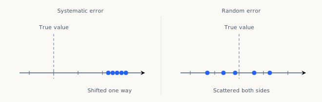
Systematic error shifts every reading to the same side of the true value; random error scatters readings on both sides of it.

1. Systematic Errors

A systematic error is a consistent, repeatable bias in one direction. It affects the accuracy of a measurement. If you took many measurements, they would all be off from the true value in the same way.

Sources: Poorly calibrated instruments (a scale that reads 1 kg when nothing is on it), environmental factors, or a consistent mistake in experimental procedure.
Correction: Can, in principle, be identified and corrected for.

2. Random Errors

A random error is an unpredictable, fluctuating error. It affects the precision of a measurement. The measurements are scattered around some mean value.

Sources: Fluctuations in the environment (a sudden draft of air), limitations in reading an instrument, inherent unpredictability in the system being measured.
Correction: Cannot be corrected for, but its effect can be reduced by taking the average of many measurements.

Quantifying Error

When the true value is known, we can quantify the error in a measurement in several ways:

Absolute Error: The absolute difference between the measured value and the true value.
$|\text{measured} - \text{true}|$
Relative Error: The absolute error divided by the true value. It is a fractional error.
$\frac{|\text{measured} - \text{true}|}{|\text{true}|}$
Percentage Error: The relative error expressed as a percentage.
$\frac{|\text{measured} - \text{true}|}{|\text{true}|} \times 100\%$

Zero Error of an Instrument

Many instruments carry a built-in error that has nothing to do with how carefully they are used. If a measuring device gives a non-zero reading even when the true value of the quantity being measured is actually zero, the device is said to have a zero error. A weighing machine that reads 0.2 kg with nothing at all on its pan, for instance, has a zero error of $+0.2$ kg — and every subsequent reading it gives is displaced by this same amount.

Zero error may be positive or negative depending on which way the instrument's reading is displaced from true zero. Once you know an instrument's zero error $Z$ , you can correct any measured reading $M$ it produces to recover the true value $T$ :

$T = M - Z$

Notice how this connects to the two error types above: a zero error is a systematic error — it displaces every single reading in the same direction by the same amount, so it can be measured once (with nothing to measure) and then subtracted out of every future reading using the formula above. This is exactly the correction procedure you will apply when reading a vernier caliper or a screw gauge.

Mean Absolute Error

The absolute/relative/percentage error formulas above all assume you already know the true value — say, a textbook constant like $g=9.81$ m/s $^2$ . But in most real experiments nobody hands you the true value in advance: even with the best possible technique, there is always some scope for random error, and all you have is a set of repeated readings taken under (hopefully) identical conditions. In that case, we adopt a working convention: the mean of the repeated readings is treated as the true value.

If $a_1, a_2, a_3, \ldots, a_n$ are $n$ repeated measurements of a quantity, the best estimate of its true value is

$a_{\text{True}} = \frac{a_1+a_2+a_3+\cdots+a_n}{n}$

Each individual reading then has its own error relative to this mean: $\Delta a_1 = a_1-a_{\text{True}}$ , $\Delta a_2=a_2-a_{\text{True}}$ , and so on. Some of these are positive and some negative — averaging them directly would mostly cancel out and hide the real scatter in the data. Instead, we average their magnitudes to get the mean absolute error:

$\Delta a_{\text{Mean}} = \frac{|\Delta a_1|+|\Delta a_2|+\cdots+|\Delta a_n|}{n}$

The final result of the experiment is then reported as $a_{\text{True}}\pm\Delta a_{\text{Mean}}$ , provided $\Delta a_{\text{Mean}}$ exceeds the least count of the instrument used. If it doesn't — the scatter in your readings is smaller than the instrument can even resolve — you instead report the result as $a_{\text{True}}\pm L$ , where $L$ is the instrument's least count.

Relative and Percentage Error, Revisited

With no external true value to compare to, the relative (fractional) error is now defined using the mean absolute error and the mean itself:

$\delta a_{\text{Relative}} = \frac{\Delta a_{\text{Mean}}}{a_{\text{True}}}$

Multiplying this by 100% expresses it, as before, as a percentage error.

Example 9: Mean Absolute Error in a Pendulum's Time Period

Problem: The following readings were taken for the time period of a pendulum:

Trial	1	2	3	4	5	6
Time Period (s)	3.62	3.58	3.60	3.66	3.68	3.56

Express the time period as $T_{\text{True}}\pm\Delta T_{\text{Mean}}$ , and find the relative error in the measurement.

Solution: The mean time period is

$T_{\text{True}} = \frac{3.62+3.58+3.60+3.66+3.68+3.56}{6}\text{ s} = 3.62\text{ s}$

The individual errors relative to this mean are $\Delta T_1=0$ , $\Delta T_2=-0.04\text{ s}$ , $\Delta T_3=-0.02\text{ s}$ , $\Delta T_4=0.04\text{ s}$ , $\Delta T_5=0.06\text{ s}$ , $\Delta T_6=-0.06\text{ s}$ . The mean absolute error is therefore

$\Delta T_{\text{Mean}} = \frac{|0|+|-0.04|+|-0.02|+|0.04|+|0.06|+|-0.06|}{6}\text{ s} = 0.04\text{ s}$

So the time period of oscillation is reported as $T=(3.62\pm0.04)\text{ s}$ . The relative error, expressed as a percentage, is

$\delta T = \frac{\Delta T_{\text{Mean}}}{T_{\text{True}}}\times100 = \frac{0.04}{3.62}\times100 \approx 1.1\%$

Now Solve: To reduce random error, an experiment measuring the weight of an object is repeated 4 times, giving 5.71 N, 5.39 N, 5.56 N, and 5.62 N. Find the true value and the percentage error in the observation.

Answer: $5.57\pm1.7\%$ N.

The accepted value for the acceleration due to gravity is 9.81 m/s². A student measures it as 10.1 m/s². What is the percentage error in the measurement?

Taking the average of many repeated readings mainly reduces the effect of which type of error?

Examples

Worked Examples: Combination of Errors

The four examples below apply the addition, multiplication/division, and power-law rules from the previous section to realistic experimental situations.

Example 10: Series Resistance

Problem: Two resistances $R_1 = 123\pm5\,\Omega$ and $R_2 = 234\pm8\,\Omega$ are connected in series. Determine the equivalent resistance of the combination.

Solution: In series, $R = R_1 + R_2$ . Since this is an addition, the absolute errors simply add:

$\Delta R = \Delta R_1 + \Delta R_2 = 5 + 8 = 13\,\Omega$

Hence the equivalent resistance is $R = (123+234)\pm13\,\Omega = (357\pm13)\,\Omega$ .

Now Solve: The lengths of two rods are $L_1 = 13.2\pm0.3$ m and $L_2 = 32.5\pm0.2$ m. Find the sum and the difference of their lengths, with errors.

Answer: Sum $= (45.7\pm0.5)$ m; difference $= (19.3\pm0.5)$ m.

Example 11: Charge on a Capacitor

Problem: The capacitance of a capacitor is $C=(20\pm1)\,\mu\text{F}$ and the applied voltage is $V=(240\pm6)$ V. Determine the charge $q$ on the capacitor using $q=CV$ .

Solution: The nominal charge is

$q = (20\,\mu\text{F})(240\text{ V}) = 4800\,\mu\text{C} = 4.8\text{ mC}$

Since $q=CV$ is a product, the fractional errors add. First, the individual percentage errors are

$\frac{\Delta C}{C}\times100 = \frac{1}{20}\times100 = 5\%, \qquad \frac{\Delta V}{V}\times100 = \frac{6}{240}\times100 = 2.5\%$

$\frac{\Delta q}{q}\times100 = 5\% + 2.5\% = 7.5\%$

The absolute error in $q$ is therefore $\Delta q = \left(\dfrac{7.5}{100}\right)(4.8\text{ mC}) = 0.36\text{ mC}$ , giving $q = (4.8\pm0.36)$ mC.

Now Solve: A current of $(2.0\pm0.1)$ A flows through a resistor of resistance $(10.0\pm0.1)\,\Omega$ . Find the potential difference $V=iR$ across the resistor, with its error.

Answer: $V = (20.0\pm1.2)$ V.

Example 12: Percentage Error in g from a Pendulum

Problem: The time period of a simple pendulum is given by $T=2\pi\sqrt{\ell/g}$ . The length of the pendulum is measured as $\ell=(10\pm0.1)$ cm and the time period as $T=(0.5\pm0.02)$ s. Determine the percentage error in the value of $g$ .

Solution: Rearranging for $g$ gives $g=\dfrac{4\pi^2\ell}{T^2}$ , so by the power-law rule,

$\frac{\Delta g}{g} = \frac{\Delta \ell}{\ell} + 2\frac{\Delta T}{T}$

The individual percentage errors are

$\delta\ell = \frac{\Delta\ell}{\ell}\times100 = \frac{0.1}{10}\times100 = 1\%, \qquad \delta T = \frac{\Delta T}{T}\times100 = \frac{0.02}{0.5}\times100 = 4\%$

$\delta g = 1\% + 2(4\%) = 9\%$

Now Solve: The mass of an object is measured as $(2.50\pm0.05)$ kg and its speed as $(4.00\pm0.02)$ m/s. Find the percentage error and the value of its kinetic energy, $K=\tfrac12mv^2$ .

Answer: Percentage error $=3\%$ ; $K=(20.0\pm0.6)$ J.

Example 13: A General Power-Law Formula

Problem: A physical quantity $x$ is calculated from the relation $x=\dfrac{a^2b^3}{c\sqrt{d}}$ . If the percentage errors in $a$ , $b$ , $c$ , and $d$ are 2%, 1%, 3%, and 4% respectively, what is the percentage error in $x$ ?

Solution: Applying the power-law rule to every factor (noting that $\sqrt{d}=d^{1/2}$ ):

$\frac{\Delta x}{x} = 2\frac{\Delta a}{a} + 3\frac{\Delta b}{b} + \frac{\Delta c}{c} + \frac{1}{2}\frac{\Delta d}{d}$

Substituting the given percentage errors,

$\delta x = 2(2\%) + 3(1\%) + 3\% + \frac{1}{2}(4\%) = 4\%+3\%+3\%+2\% = 12\%$

Now Solve: A physical quantity $x$ is calculated from the relation $x=\dfrac{\sqrt{a}}{b^2c}$ . If the percentage errors in $a$ , $b$ , and $c$ are 1%, 0.5%, and 2% respectively, what is the percentage error in $x$ ?

Answer: 3.5%.

In $g = \dfrac{4\pi^2\ell}{T^2}$ , the percentage errors in $\ell$ and $T$ are 2% and 3% respectively. What is the percentage error in $g$ ?

Introduction to Experimental Skills

Physics begins with measurement, and no measurement is exact. This chapter builds the skills needed to handle that fact honestly: counting significant figures and rounding correctly, telling accuracy apart from precision, classifying and combining experimental errors, and reading two classic precision instruments, the vernier caliper and the screw gauge.

Length Measuring Instruments: Vernier Caliper and Screw Gauge

Reading an Instrument: Least Count and Zero Error

Every measuring instrument has a natural limit to how finely it can resolve a reading — this is called its least count: the smallest value of a quantity that the instrument can measure accurately, essentially set by the value of its smallest scale division. A metre ruler with millimetre markings has a least count of 1 mm; the vernier caliper and screw gauge you will meet below are specifically engineered to push this limit far smaller, without needing impossibly fine markings.

You should also recall the idea of zero error from the previous section: if an instrument gives a non-zero reading when there is genuinely nothing to measure, every reading it produces is displaced by that same amount, and must be corrected using $T = M - Z$ before it can be trusted. Keep both ideas in mind as you read on — least count tells you how finely you can read an instrument, while zero error tells you whether its scale is honestly lined up with true zero in the first place. Both the vernier caliper and the screw gauge require you to apply each of these ideas explicitly.

The Ruler

The simplest length-measuring instrument is the ordinary ruler. To measure the length of an object, you read the ruler's mark at each end and take the difference between the two readings.

A rod placed against a ruler, with its two ends read against the centimeter scale

In the diagram, we read the greatest scale mark at end A and at end B of the rod. The difference between these two readings gives the length of the rod as $14\text{ cm}\pm1\text{ cm}$ — the $\pm1\text{ cm}$ reflects the least count of the ruler, and gives the maximum and minimum lengths consistent with what could actually be read off the scale. A ruler's precision is capped by the width of its smallest division; to do better without needing impossibly fine markings, we need an instrument that multiplies our reading precision by comparing two mismatched scales — this is exactly what the vernier caliper achieves.

The Vernier Caliper

Construction: Two Scales, Slightly Mismatched

A vernier caliper consists of two scales sitting side by side. The main scale is a standard ruler-like scale with divisions of a fixed, familiar length (typically 1 mm or 1 cm). Alongside it slides a second, shorter vernier scale, whose divisions are made deliberately slightly different in length from the main scale's divisions — and this deliberate mismatch is the entire trick behind the instrument's extra precision.

The vernier and main scales with their zero marks aligned, showing how the divisions of each scale drift apart

Suppose ten divisions of the vernier scale span the same length as nine divisions (of 1 cm each) of the main scale, with both zero marks initially coinciding. Then a single vernier division is shorter than a single main-scale division by

$1\text{ cm} - \frac{9\text{ cm}}{10} = 0.1\text{ cm}$

This small mismatch accumulates steadily: after the 2nd division the two scales have drifted apart by $2\times0.1\text{ cm}=0.2\text{ cm}$ , after the 3rd by $0.3\text{ cm}$ , and so on — until, after all ten divisions, the accumulated drift totals exactly $1\text{ cm}$ , bringing the vernier scale's last mark back into coincidence with the main scale's 9 cm mark.

Reading a Length

To measure the length of a rod AB with this pair of scales, we align the zero of the main scale with end A and the zero of the vernier scale with end B.

A rod slightly longer than 5 cm, whose vernier zero has slid past the 5 cm mark until the 4th vernier division lines up exactly with the 9 cm main-scale mark

In the diagram, the rod is evidently a little longer than 5 cm. Had the vernier's zero landed exactly on the 5 cm mark, the vernier's 4th division would have sat 0.4 cm away from the main scale's 9 cm mark (since each division differs by 0.1 cm). Instead, the two coincide exactly — which tells us the vernier's zero has slid 0.4 cm past the 5 cm mark. The rod's length is therefore 5.4 cm. This coincidence trick lets the instrument resolve lengths down to 0.1 cm even though neither scale on its own is marked that finely — so 0.1 cm is the least count of this particular caliper.

The General Least-Count Formula

The reasoning above generalizes directly. If $N$ divisions of the vernier scale are made to span the same length as $N-1$ divisions of the main scale, then

$N\times(\text{vernier scale division}) = (N-1)\times(\text{main scale division})$

Rearranging,

$\text{main scale division} - \text{vernier scale division} = \frac{\text{main scale division}}{N}$

The left-hand side is exactly the least count $L$ of the instrument — the smallest length it can resolve via a single coincidence. So if $m$ is the length of one main-scale division,

$L = \frac{m}{N}$

The Reading Formula

Once you know $L$ , reading the instrument is a two-step process: read the main-scale reading $M$ — the last main-scale mark that the vernier's zero has crossed — then find which vernier division $k$ coincides exactly with some main-scale mark. The full reading is

$R = M + kL \pm L$

where the trailing $\pm L$ reflects the least count as the uncertainty in the reading, exactly as it did for the plain ruler above. Always remember to check the caliper's zero error before trusting a reading, and correct it using $T=M-Z$ if needed.

A complete vernier caliper with its jaws, main scale, and vernier scale, measuring the diameter of a sphere held between the jaws

Example 14: Least Count of a Vernier Caliper

Problem: A vernier caliper has 1 mm marks on its main scale. It has 20 equal divisions on its vernier scale, which match with 16 main-scale divisions. Find the least count of this caliper.

Solution: Since 20 vernier scale divisions (VSD) span the same length as 16 main scale divisions (MSD),

$1\text{ VSD} = \frac{16}{20}\text{ MSD} = \frac{4}{5}\text{ MSD}$

The least count is the difference between one main-scale division and one vernier-scale division:

$L = 1\text{ MSD} - 1\text{ VSD} = \left(1-\frac{4}{5}\right)(1\text{ mm}) = 0.2\text{ mm}$

Now Solve: A vernier caliper has 1 mm marks on the main scale, and 20 equal divisions on the vernier scale that match with 18 main-scale divisions. Find its least count.

Answer: 0.1 mm.

Example 15: Reading a Vernier Caliper

Problem: State the diameter of the sphere as measured by the vernier caliper shown below.

A vernier caliper measuring a sphere, with the vernier scale zoomed in to show the coinciding division

Solution: The least count of this caliper is $\dfrac{1}{10}(1\text{ mm}) = 0.01\text{ cm}$ . The main scale reading is $M = 1.3\text{ cm}$ , and the 3rd vernier division is the one that coincides exactly with a main-scale mark, so $k=3$ . The reading is

$R = 1.3\text{ cm} + 3\times\frac{1}{10}(1\text{ mm}) = 1.33\text{ cm}$

Reporting the least count as the uncertainty, the diameter of the sphere is $(1.33\pm0.01)\text{ cm}$ .

Now Solve: Find the reading of the vernier caliper shown below.

A second vernier caliper reading, to be worked out independently

Answer: 3.44 cm.

The Screw Gauge

Construction: Pitch and Circular Scale

A screw gauge (or micrometer screw) uses a precisely threaded rod that advances along its own axis as it is rotated — exactly like a screw. The distance the rod advances in one complete rotation is called the pitch of the screw gauge, and it sets the value of the main linear scale. A circular scale attached to the rotating thimble is divided into a large number of equal parts, letting you read off the fraction of a rotation completed beyond the last whole pitch.

The frame of a screw gauge showing the threaded spindle, the linear (pitch) scale, and the rotating circular scale

If the length of one pitch is $m$ and the circular scale has $N$ divisions, then one division of the circular scale corresponds to an axial advance of

$L = \frac{m}{N}$

and this $L$ is the least count of the screw gauge — the same reasoning that gave the vernier caliper's least count, applied to a rotating rather than a sliding scale.

Reading a Screw Gauge

To read a screw gauge, count the number of complete pitches $M$ the spindle has advanced (read off the linear scale), then read the division $k$ on the circular scale that lines up with the linear scale's reference line after the last complete pitch. The full reading is

$R = M(m) + k(L) \pm L$

where, once again, the trailing $\pm L$ is the least count reported as the reading's uncertainty. As with the vernier caliper, always check for zero error before trusting a screw gauge's reading — if the spindle reads a non-zero value when fully closed with nothing between its faces, that constant offset must be subtracted from every subsequent reading using $T=M-Z$ .

A screw gauge with the spindle closed on a wire, showing the linear scale reading and the aligned circular scale division

Example 16: Least Count of a Screw Gauge

Problem: A screw gauge has a pitch of 1 mm and 50 divisions on its circular scale. Find its least count.

Solution:

$L = \frac{1\text{ mm}}{50} = 0.02\text{ mm}$

Now Solve: A screw gauge has a pitch of 2 mm and 100 divisions on its circular scale. Find its least count.

Answer: 0.02 mm.

Example 17: Reading a Screw Gauge

Problem: Ten rotations of a screw gauge's cap correspond to 5 mm, and the cap has 100 divisions. Find the least count. A reading taken for the diameter of a wire shows four complete rotations, plus 35 divisions on the circular scale beyond that. Find the diameter of the wire.

Solution: One rotation corresponds to a pitch of $m = \dfrac{5\text{ mm}}{10} = 0.5\text{ mm}$ , so the least count is

$L = \frac{0.5\text{ mm}}{100} = 0.005\text{ mm}$

With $M=4$ complete rotations and $k=35$ circular-scale divisions,

$R = 4(0.5\text{ mm}) + 35(0.005\text{ mm}) = 2.175\text{ mm}$

The diameter of the wire is 2.175 mm.

Now Solve: A screw gauge of least count 0.01 mm and pitch length 2 mm is used to measure the thickness of a book. The measurement shows 4 rotations and 23 divisions on the circular scale. Find the thickness of the book, and state how many divisions are on the circular scale.

Answer: 8.23 mm; 200 divisions.

A vernier caliper's zero error is +0.02 cm (the vernier zero reads past the main-scale zero when the jaws are closed). A measurement gives a raw reading of 2.55 cm. What is the corrected (true) length?

On a vernier caliper, 10 vernier divisions span the same length as 9 main-scale divisions of 1 mm each. What is the least count of the instrument?

Precision, Accuracy, and Error Calculations

Accuracy vs. Precision

In everyday language, accuracy and precision are often used interchangeably. In science, they mean very different things. Understanding the difference is crucial for evaluating the quality of experimental data.

Accuracy is how close a measurement is to the true or accepted value. An accurate measurement has low systematic error.
Precision is how close a set of repeated measurements are to each other. A precise measurement has low random error.

The Dartboard Analogy

A common and effective way to visualize the difference is to think of a dartboard. The bullseye represents the 'true' value you are trying to measure.

Four dartboards comparing accuracy and precision. The centre of each board is the true value.

High Accuracy, High Precision: The darts are clustered tightly in the bullseye. This is the ideal result.
Low Accuracy, High Precision: The darts are clustered tightly together, but they are far from the bullseye. This often indicates a systematic error, like a misaligned scope.
High Accuracy, Low Precision: The darts are spread out, but their average position is in the bullseye. This often indicates significant random error.
Low Accuracy, Low Precision: The darts are spread out all over the board, far from the bullseye.

Consider a dartboard where the darts are all clustered in a tight group in the top-left corner, far from the bullseye. What does this represent?

A student's repeated measurements agree closely with one another but are all consistently far from the true value. Which type of error is most likely responsible?

Rounding and Operations with Significant Figures

The 'Weakest Link' Principle

When you perform calculations with measured numbers, the result cannot be more precise than your least precise measurement. Think of it like a chain: its strength is determined by its weakest link. In calculations, the 'weakest link' is the number with the least certainty.

This means we must round our final answer to reflect this uncertainty. The rules for rounding depend on the type of operation you're performing.

The Rules of Calculation

There are two distinct rules for rounding, depending on whether you are adding/subtracting or multiplying/dividing.

Addition and subtraction: round the result to the same number of decimal places as the term with the fewest decimal places.
Multiplication and division: round the result to the same number of significant figures as the factor with the fewest significant figures.

Rounding Rules

When rounding to the correct number of digits:

If the first digit to be dropped is 4 or less, simply drop it and all following digits.
If the first digit to be dropped is 5 or greater, increase the last retained digit by one.

Example: rounding 1.2346 to three significant figures gives 1.23; rounding it to four gives 1.235.

Example 8: Perimeter and Area to the Correct Significant Figures

Problem: The length and breadth of a rectangle are measured as 3.61 cm and 2.1 cm. State its perimeter and area to the proper number of significant figures.

Solution: Perimeter is found by addition, so we round by decimal places (the fewest decimal places among the terms being added is one, from 2.1 cm):

$\text{Perimeter} = 3.61\text{ cm} + 2.1\text{ cm} = 5.7\text{ cm}$

Area is found by multiplication, so we round by the fewest total significant figures (2.1 cm has only two):

$\text{Area} = 3.61\text{ cm}\times2.1\text{ cm} = 7.6\text{ cm}^2$

Now Solve: Two resistors of resistance 12 $\Omega$ and 20.2 $\Omega$ are connected in series. What is their equivalent resistance, to the correct number of significant figures?

Answer: 32 $\Omega$ .

The Special Case: Rounding Off a Trailing 5

The basic rule above is clear when the digit to be dropped is above or below 5 — but what happens when it is exactly 5, with nothing but zeros after it? Always rounding this case up would introduce a small systematic bias into your data, since over many roundings values would drift upward more often than downward. To keep rounding statistically unbiased, physicists use the round-half-to-even convention for this special case:

If the digit to be dropped is 5 (and the digit before it is the one being retained) and that retained digit is already even, the 5 is simply dropped and the retained digit is left unchanged.
If the retained digit is odd, it is raised by one — which makes it even.

Either way, the retained digit ends up even. This convention (sometimes called "banker's rounding") ensures that, averaged over many measurements, rounding up and rounding down happen equally often.

Order of Magnitude

Physics regularly deals with quantities spanning an enormous range of scales — the size of a mountain versus the size of a pin's tip, or the mass of a galaxy versus the mass of a single hydrogen atom. Comparing such wildly different numbers digit by digit is unwieldy; instead we ask a coarser question: roughly what power of ten is this number closest to? That power is the number's order of magnitude.

To find it, write the number in scientific notation as

$N \times 10^{x}$

where $1 \le N < 10$ and $x$ is an integer. Then round the coefficient $N$ itself to either 1 or 10: if $N \le 5$ , round it down to 1; if $N > 5$ , round it up to 10. The number is then approximately $10^{x}$ or $10^{x+1}$ , so its order of magnitude is $x$ (when $N \le 5$ ) or $x+1$ (when $N > 5$ ).

For example, the speed of light $c = 3\times10^{8}$ m/s has an order of magnitude of 8, since $3 \le 5$ . Avogadro's number $N_A = 6.023\times10^{23}$ has an order of magnitude of 24, since $6.023 > 5$ .

Example: Order of Magnitude and Rounding — The Height of Everest

Problem: The height of Mount Everest is 8815 m. What is the order of magnitude of this height? Also round off the given height to three significant figures.

Solution: Writing the height in scientific notation:

$8815\text{ m} = 8.815\times10^{3}\text{ m}$

The coefficient 8.815 is greater than 5 (it is, in fact, close to 10), so the order of magnitude is $3+1=$ 4.

Now round 8815 m to three significant figures. We must decide between 8810 m and 8820 m — the digit being dropped is exactly 5, and the digit before it is '1', which is odd. By the round-half-to-even rule, an odd retained digit is raised by one to become even, so '1' becomes '2', and we round to 8820 m (since 2 is even).

Now Solve: What is the order of magnitude of your own height, expressed in centimeters?

Answer: 2 — a height of roughly 170 cm is $1.7\times10^{2}$ cm, and since $1.7 \le 5$ , the order of magnitude is 2.

Calculate $(2.5 \times 3.42) + 1.007$ to the correct number of significant figures.

Round 2.45 to two significant figures, following the convention used in this chapter.

Significant Figures

Communicating Certainty in Measurement

Every measurement has a degree of uncertainty. If you measure a length with a ruler, you might be certain about the millimeters, but less certain about fractions of a millimeter. Significant figures are the digits in a measured number that are known with certainty, plus one uncertain (estimated) digit. They are a shorthand way to communicate the precision of your measurement.

For example, writing a length as $12.3$ cm implies that the '1' and '2' are certain, while the '3' is an estimate. Writing $12.30$ cm implies a more precise measurement, where you are certain of the '1', '2', and '3', and the '0' is the estimated digit.

The Rules for Counting Significant Figures

To read and write numbers correctly, we use a standard set of rules to determine which digits are significant.

All non-zero digits are significant.
Zeros between non-zero digits are significant.
Leading zeros are not significant; they only fix the position of the decimal point.
Trailing zeros after a decimal point are significant.
Trailing zeros in a whole number written without a decimal point are not significant.

The Ambiguous Case: Trailing Zeros

For a number like 5000, it's unclear if the measurement is precise to the thousands place (1 sig fig) or all the way to the ones place (4 sig figs). To remove this ambiguity, we use scientific notation.

$5 \times 10^3$ clearly has 1 significant figure.
$5.0 \times 10^3$ clearly has 2 significant figures.
$5.000 \times 10^3$ clearly has 4 significant figures.

Example 7: Counting Significant Figures

Problem: Mention the number of significant figures in the following measured values of an experiment: (i) 430 m (ii) 0.320 N (iii) $4.83\times10^3$ kg (iv) 4.9080 cm $^3$

Solution:

(i) 430 m has two significant figures — a trailing zero in a number written without a decimal point is not significant.
(ii) 0.320 N has three significant figures — the leading zero is only a placeholder, but the trailing zero after the decimal point is significant.
(iii) $4.83\times10^3$ kg has three significant figures — only the digits in the coefficient are counted.
(iv) 4.9080 cm $^3$ has five significant figures — every digit, including the trailing zero after the decimal point, is significant.

Now Solve: How many significant digits are there in 1.090 m?

Answer: Four.

How many significant figures are in the measurement 0.02050 meters?

A measurement is reported as 1,200,000 km. How would you write this in scientific notation to unambiguously show it has exactly 3 significant figures?

Trial

Time Period (s)

3.62

3.58

3.60

3.66

3.68

3.56